MS Excel provides tons of dazzling data validation techniques in order to help you keep your data legitimate and refined.
In the previous article we highlighted some basic validation formula with examples. To let you get a bit deeper dive into it, we’re going to explain a couple of more advanced validation features. You’ll find them quite useful on many occasions while constructing your worksheets. So let’s move ahead.
Validate If The Value Exists in The Given List
Here we’re going to explain how to create a range of cells having values only matching from another range of cells. Hence the user will be able to ensure that there’s no invalid/not-allowed value in the range of specified cells.
In the example shown, the data validation applied to A3:A11 is:
=COUNTIF(ValidFruites,A3)>0
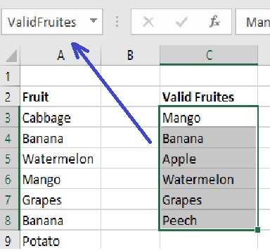
Where ValidFruites is the name of a cell range (here C3:C8) which contains name of some delicious fruits. In order to define a name for a specified range spot and click Formulas -> Define Names -> Define Name.

If you select this range any time you can see the name of the range in the box on the top-left corner as shown in the image below.

At this point you’re all set to define a range of cells to be validated against another range.
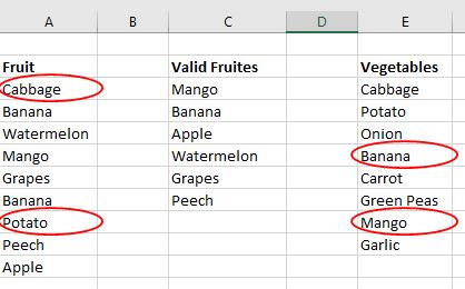
You can apply data validation to cells that already have data entered in them. However, Excel does not automatically notify you that the existing cells contain invalid data. In this scenario, you can highlight invalid data by instructing Excel to circle it on the worksheet. Once you have identified the invalid data, you can hide the circles again. If you correct an invalid entry, the circle disappears automatically.
To apply the circles, select the cells you want to evaluate and click Data > Data Tools > Data Validation > Circle Invalid Data.
Validate If The Value Does Not Exist in The Given List
In the above example we validated that the values in a cell range should match a given list (ValidFruites). There are occasions when we’re required to validate if the values in a cell range should be other than those in a given list. This can be accomplished in the same manner as above but with a slight difference.
Suppose we’re having name of some vegetables in a cell range and obviously we do not want the user to enter a name of a fruit in this range. So instead of the validation formula like
=COUNTIF(ValidFruites,A3)>0
we’ll use a formula like
=COUNTIF(ValidFruites,E3)=0
Where E3 is the first cell of our vegetables range and the operator “=” is used instead of “>”. This dictates that our vegetables cell value should not belong from the ValudFruites range.
Note that we’ve already mentioned in the previous article about how to create a validation formula for one cell and then copy it to the other cells of the range in question.
In order to Encircle all invalid values, again select the cells you want to evaluate and click Data > Data Tools > Data Validation > Circle Invalid Data
and voila! you’ll see exactly what you expected. This amazing feature helps you to keep your excel sheet’s data refined.


