In Microsoft Excel, an Array Formula provides you with a way to do powerful calculations on one or more value sets. The Array Formula works with an array of values, rather than a single value. Array formulas can return a single result, or multiple results. That sounds pretty simple enough, and indeed many array formulas are quite straight forward.
In fact, the role of array formula, is to perform magic. In the hands of an Excel master, array formulas get the right answers in complex situations, such as fulfilling multiple criteria, where ordinary Excel users have given up because the problem is “unsolvable”.
The array formula returns an array of values. That resultant array may be passed to another function that is expecting an array of inputs. If so, that function returns its normal single value result. It is up to the user to use array formulas to extract the required result in a particular form; array or a single value.
Array formulas are frequently used for data analysis, conditional statistical calculations like sum, average, count and lookups, linear algebra, matrix math and manipulation, and much more. Don’t worry! we’re not going to do anything complex here.
So let’s roll up our sleeves and start with a pretty simple example.
1- A Hard-Coded Array
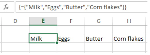
Let’s fill a range of cells in a row with an array. Select four adjacent cells in a row and then enter this in the formula bar:
={“Milk”,”Eggs”,”Butter”,”Corn flakes”}
Remember! The Array Formula is a special type of formula that must be entered by pressing Ctrl+Shift+Enter. The formula bar will show the formula surrounded by curly braces like {=…}. So what you have to do is, while the cursor is on formula bar press Ctrl+Shift+Enter keys at the same time (press and hold Ctrl then press and hold Shift and then press Enter key and lift your all three fingers immediately, it’s that easy!) and see the little magic in the current cell.
2- Let’s Advance a Little
Fill the cells as shown in the picture below. Move to the cell after Total Sale and enter this array formula in the formula bar:
=SUM(Q25:Q28*R25:R28)
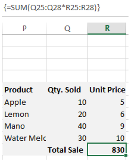
Make it the array formula by pressing Ctrl+Shift+Enter and what you see in the current cell will be the sum of the product of the Quantity * Unit Price, that is, total sales. Although you can get it without using array formula by adding another column and calculating individual sales and summing up that column in this one. But anyways, this is how you can achieve the same thing without using extra columns.
Another function MAX() does well using array formula. Similar to above fill the cells as shown in the picture below. Move to the cell below Max. Diff. and enter this array formula in the formula bar:
=MAX(D5:D11-C5:C11)
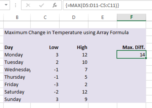
The result will show the maximum change in the temperature. Not to mention that if you’re well comfortable with array formula syntax which frequently uses cell ranges then you will want to provide your own range based on where you have placed your data.
3- Place a Matching Row
Given quarterly sales against various regions, let’s display the row of the specific region, as well as, the minimum sales and the sum of all quarters for that region.
Place this table across B to F columns. Enter Region of your choice (e.g, South) in the cell H16. Select four adjacent cells H17:K17 and enter this formula in the formula bar:
=INDEX(C16:F19,MATCH(H16,B16:B19,0),0)

Make it the array formula by pressing Ctrl+Shift+Enter. Now you’ll see the magic! The current range of cells will contain the row belonging to the selected region. Change the region to Central and the cells below it will immediately update with the row belonging to Central region.
Now select cell H21 and enter this formula:
=MIN( INDEX(C16:F19,MATCH(H16,B16:B19,0),0))
You don’t have to make it array formula. What you’ll see in this cell is self-explanatory, that is, it will show the minimum value belonging to that region.
Likewise enter this formula in the cell I21:
=SUM(INDEX(C16:F19,MATCH(H16,B16:B19,0),0))
You don’t have to make it array formula. It will show the total of all quarters of that region.
4- Conditional Sum Based on One or More Parameters
Build the data of the first four columns, as in the below image in your excel sheet. Remember to start from B33 and it should end up on E40. This is required because when you copy/paste the array formula you’ll see the results immediately. When you comprehend it, you can place your data anywhere on your sheet but you have to adjust the cell ranges in your formula accordingly.
Now enter a region like North in the cell G34. Enter this formula in the cell H34, right after G34.
=SUMIFS(E34:E40,C34:C40,G34)
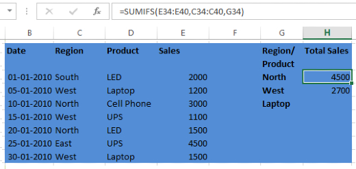
Note that this is not an array formula. What it does, it summs up sales amounts (E34:E40) filtered on region (C34:C40) by the value G34, which is North at the moment. So it will sum up sales of North region that is (3000+1500) = 4500. Pretty simple, isn’t it?
Let’s make it some more complicated. Just kidding!
Enter West below North and Laptop below West. Now enter this formula ahead of West:
=SUMIFS(E34:E40,C34:C40,G35,D34:D40,G36)
Again this is not an array formula. What it does, it Sums up all sales of ‘Laptop’ in the region ‘West’. See for yourself.
May be you won’t be much convinced using these rather complex functions at the moment, but in fact, you’ll be awe-inspired when your data is pretty large spanning thousands of rows.
5- Conditional Statistics Functions
Let’s move on with something real interesting. Enter the values taken from Date, Sales Rep. and Sales columns in the cells starting from P34.
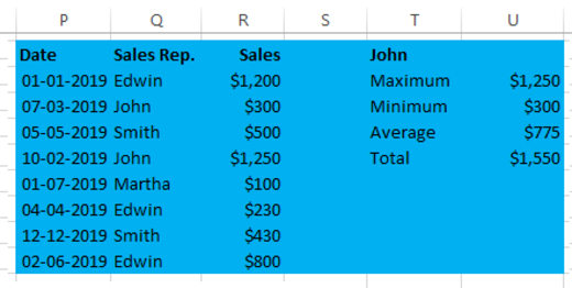
Place your cursor at T34. Now we’re going to make it a drop-down whose values will come from Sales Rep. column. This will make it easy to select any sales rep. instead of typing their name. While you remain in T34:
Click Data tab from the top menu.
Click Data Validation from Data Tools Group
On the Settings tab, in the Allow box, Select List.
In the Source box, type in your List values like “$Q$35:$Q$42” in our case because we want the list to populate from Sales Reps.
Finally make sure that the In-cell drop-down check box is selected. Click Ok and you’re done.
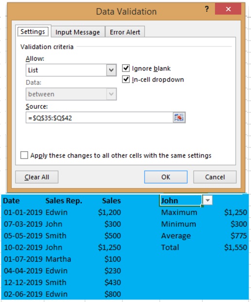
Select a Sales rep. like Edwin from our created drop-down. Enter Maximum in the cell right below it.
Place your cursor in U35, adjacent to Maximum and enter this formula in it:
=MAX(IF($Q$35:$Q$42=$T34, $R$35:$R$42))
Make it the array formula by pressing Ctrl+Shift+Enter. This formula filters the Sales Rep. $Q$35:$Q$42 by the value in T34 (Edwin), and returns the maximum value from Sales column.
Now perform the same to get minimum. Things are intuitive for you so we’ll only mention the formula to get minimum value.
=MIN(IF($Q$35:$Q$42=$T$34, $R$35:$R$42))
Which resembles the above formula.
Now get the total using SUM() formula:
=SUM(IF($Q$35:$Q$42=$T$34, $R$35:$R$42))
Now see the little magic by selecting some other Sales Rep. e.g, John and you should observe that all statistical values will display data about John. Now again this functionality is quite handy when the data is large enough and the user has to quickly observe the performance of the typical sales reps.

