
Microsoft Excel provides a very powerful formula language. You can achieve amazing things if you’re well capable of using it.
Here’s the calculation of some of the public holidays in USA. You can calculate the rest in the same manner.
Place the years in column A. Please refer to the below images taken from the Excel sheet.
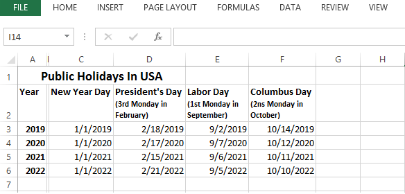
Here are the formula for some of the official holidays in USA:
New Year Holiday
Pretty simple. It should be 1st January of the year in question.
Assuming we are on C3 cell, so the formula to calculate New Year will be
=DATE(A3,1,1)
Where A3 is the value placed in the cell A3, that is, the year 2019. The second parameter is the month, that is, 1 means January and the third parameter is the day of the month, that is, 1.
The pretty cool thing is that you can copy the value (that is the formula) form this cell and paste in the cells below for the rest of the years and here you go.
President’s Day
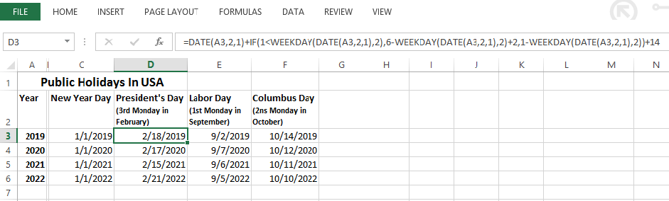
The President’s day occurs in the 3rd Monday in February. The formula appears to be a bit complex when you see it at a glance, but its quite straight-forward when you make a little effort to comprehend it.
Assuming we are on D3 the formula is as below.
=DATE(A3,2,1)+IF(1<WEEKDAY(DATE(A3,2,1),2),6-WEEKDAY(DATE(A3,2,1),2)+2,1-WEEKDAY(DATE(A3,2,1),2))+14
The Date() function returns the date given the year (here it is in cell A3), month (here it is February) and the day of the month (here it is 1).
The formula here on till “+14” calculates the date on the 1st Monday of this month. Note that the Weekday function returns the day of the week (1-7) given the date and a flag (here it is 2, which means that Monday is the first day of the week).
Now since we are looking for the 3rd Monday so after getting the first Monday we have to add 2 weeks, that is, 14 days to reach the date at the third Monday.
Labor Day
The Labor day occurs in the 1st Monday in September. The formula is almost the same as above except a couple of things explained below.
Assuming we are on E3 the formula is as below.
=DATE(A3,9,1)+IF(1<WEEKDAY(DATE(A3,9,1),2),6-WEEKDAY(DATE(A3,9,1),2)+2,1-WEEKDAY(DATE(A3,9,1),2))
The Date() function returns the date given the year (here it is in cell A3), month (here it is September) and the day of the month (here it is 1). The formula here calculates the date on the 1st Monday of this month.
Now since we are looking for the 1st Monday so after getting the first Monday we have to add nothing at the end to reach the date at the 1st Monday.
Columbus Day
The Columbus day occurs in the 2nd Monday in October.
Assuming we are on F3 the formula is as below.
=DATE(A3,10,1)+IF(1<WEEKDAY(DATE(A3,10,1),2),6-WEEKDAY(DATE(A3,10,1),2)+2,1-WEEKDAY(DATE(A3,10,1),2))+7
The Date() function returns the date given the year (here it is in cell A3), month (here it is 10, that is, October) and the day of the month (here it is 1).
The formula here on till “+7” calculates the date on the 1st Monday of this month.
Now since we are looking for the 2nd Monday so after getting the first Monday we have to add 1 week, that is, 7 days to reach the date at the 2nd Monday.