In the previous post Excel Technique: How To Create Pivot Table about creating Pivot tables in Excel we’ve elaborated how to create
simple Pivot tables in Excel. In the current article we’re moving some further to create Pivot Charts using Pivot Tables.
A Pivot chart is a shiny diamond added to MS Excel’s crown. It is a built-in feature of MS Excel and also is a visual representation of a Pivot Table.
Lets unveil the beauty of Pivot Charts by resuming our previous job Excel Technique: How To Create Pivot Table about creating Pivot tables and create Pivot charts from those tables.
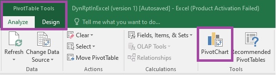
Click anywhere on the Category Pivot table. Pivot Table menu will appear in the Menu Bar. Click on Analyze Tab on the Menu Bar, and further click on Pivot Chart under Tools section.
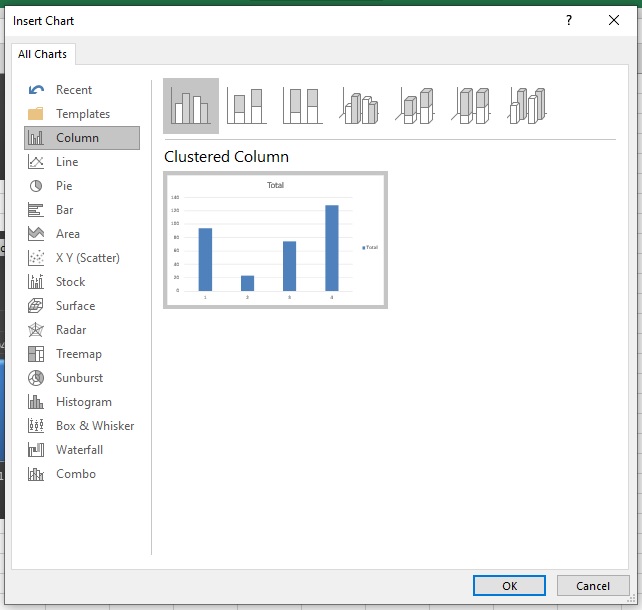
The Insert Chart dialog box will appear as shown in the below image. There’re numerous chart types you can choose from.
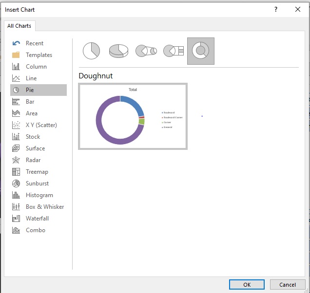
For now click Pie and then select Doughnut from the top row as shown in the image. Click Ok. A simple Pie Chart box will be placed close to the Pivot Table as shown below.
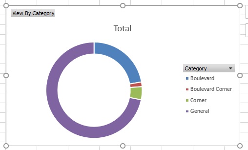
Now we need to setup a few things to make our Pivot chart some good looking and useful. Click anywhere on the Pie Chart and you’ll see two small icon boxes along the top-right edge of the chart.
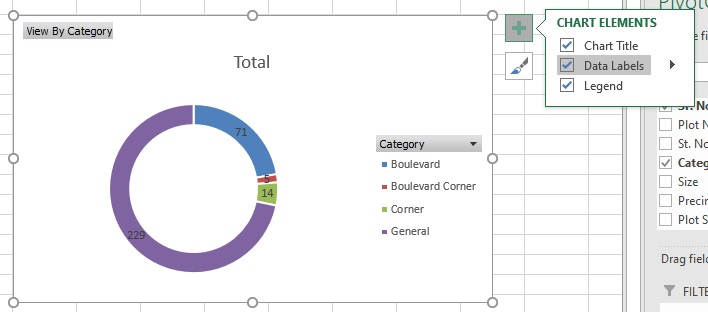
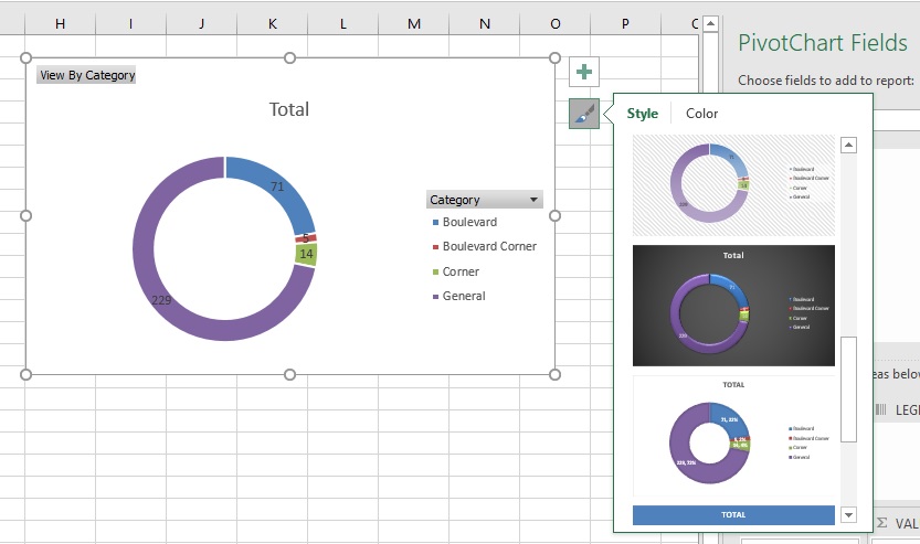
Click the second one (Style) and then choose any style that you like. For now choose the one as shown in the image below. You’ll notice that the chart style will immediately change as per your choice.
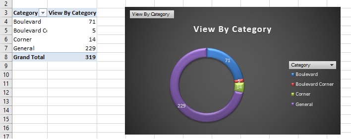
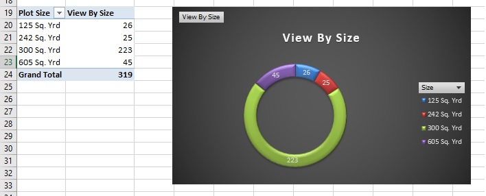
Repeat the same steps to create Pivot Charts for Size and Development Status Pivot Tables.
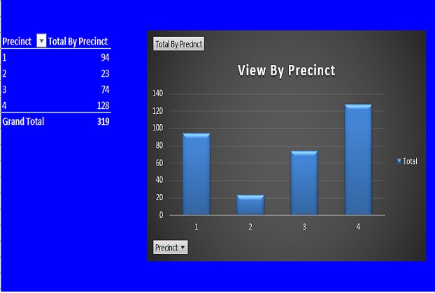
For Precinct Pivot Table let’s select a different chart. Select Column Chart from Insert Chart box.
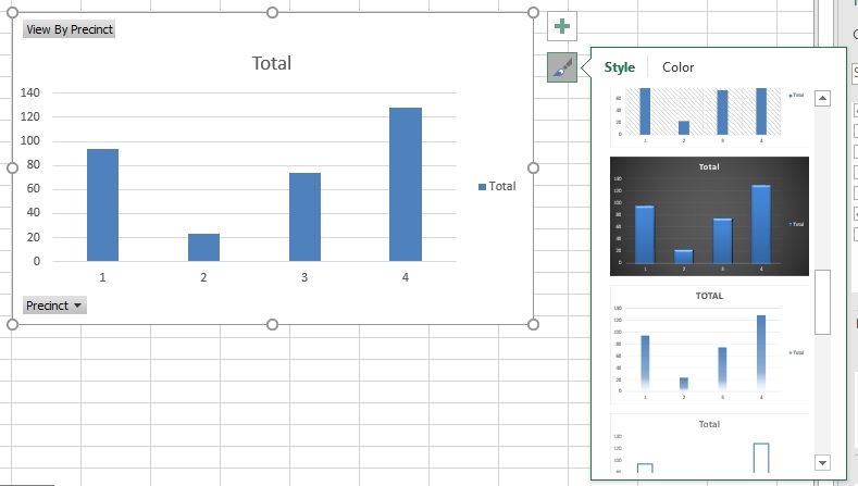
Select Style and let it be placed alongside Precinct Pivot Table, as shown in the below image.
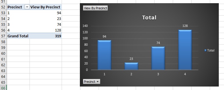
Now your Pivot Charts with their respective Pivot Tables will be shown something like the image below.

Looks pretty and useful, isn’t it?
Now as you may already be familiar with how to create slicers for each Pivot table and setup slicers to reflect immediate changes in all Pivot Tables Pivot Charts, the time has arrived to behold the magic. Just make selection from any slicer and you’ll notice that all Pivot Tables and Charts will immediately filter the data as per your selection.
But this is just the tip of the iceberg, you can create numerous Charts with a myriad of verities and options to choose.